Excel For SEOs – How To Speed Up Common Tasks

Working in SEO (or digital marketing in general), we’re constantly manipulating large data sets from a range of sources, and inevitably find ourselves deep in Excel spreadsheets. Excel is a fantastic tool for dealing with data and is pretty much essential for a lot of pretty standard SEO tasks from keyword research and opportunity analysis to formatting page titles and uncovering issues with XML sitemaps.

But it can also feel somewhat overwhelming for beginners and can continue to frustrate more advanced users who may be pretty sure the task they’re working on could be made easier by Excel, but are not 100% sure exactly how. Plus, we’re continually finding little tricks and tips that can help speed up the tasks we’re working on, which can really improve productivity with common, repetitive tasks.

So we’ve put together a series of blog posts on using Excel to complete common SEO tasks as quickly and efficiently as possible, starting with some more simple applications before working towards more complex examples. There are so many uses for Excel, so we’ll likely be adding to this list over time – if you have any further tips you want to share, or are working through a problem that you think Excel should be able to help with, get in touch and we’ll do our best to add them to the list in future.

So with this in mind, we’re going to start our series with Part 1 – Using the =CONCATENATE formula to combine URL strings and make keyword research easier.

 

The =CONCATENATE Formula – Combining Strings Of Text

Excel’s =CONCATENATE formula is pretty simple, but very effective for SEOs. All it does is combine two text strings together, but this can be very valuable when dealing with large data sets, particularly for URL strings, and for keyword research.

Using =CONCATENATE to clean URL strings in Google Analytics data

If, like most SEOs, you’ve found yourself downloading page-level data from GA, you’ll know it arrives as a CSV without the domain included:

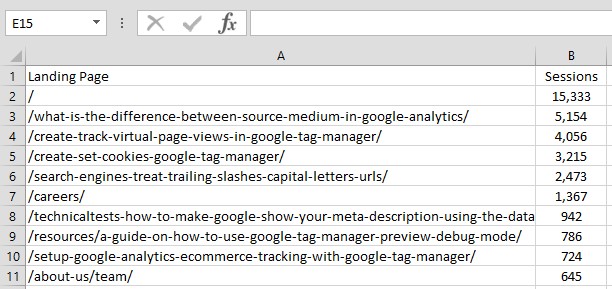
This can be frustrating, particularly if you’re looking to combine it with another data source or look up data from another list of full URLs, from Screaming Frog for example.

But =CONCATENATE can easily append the domain to each URL in your list with by adding the domain path into a separate cell in your workbook and referencing that cell in the =CONCATENATE formula.

In the example below, our domain is in cell C2 and the first URL string is in cell A2, so the basic formula would be =CONCATENATE(C2,A2):

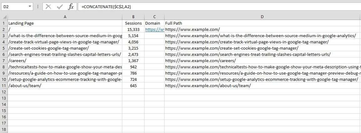
In this instance, you’d want to ‘fix’ the domain in the C2 cell in place (highlight the cell, hit F4) to ensure the =CONCATENATE formula always references the text string in this cell once you drag the formula in D2 down. This would change the formula to: =CONCATENATE($C$2,A2).

Alternatively, you can just type the text string you want to add to the URLs in column A directly into the formula, ie: =CONCATENATE(“https://www.example.com”,A2). Just make sure you put the text string you want to use within speech marks, and it will be combined with the string in A2, and can then be dragged down and applied to all cells in column A.

 

Using =CONCATENATE to make keyword research faster and easier

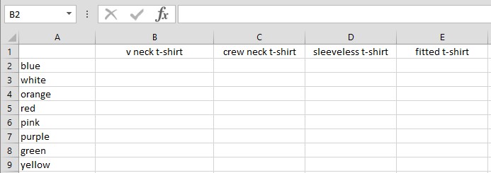
=CONCATENATE can also be very useful for keyword research. For example, you may have an ecommerce site with a whole load of different clothes products, in a range of colours. Getting a list of all combinations of clothing type and colour can get pretty complicated and time consuming, but a little concatenation can speed things up no end.

Just put one set of variables in each Row of Column A, and the other set in each Column of Row 1 as below:

Then you can start concatenating, starting in cell B2, and drag the formula down to get all colour iterations for your v neck t-shirt:

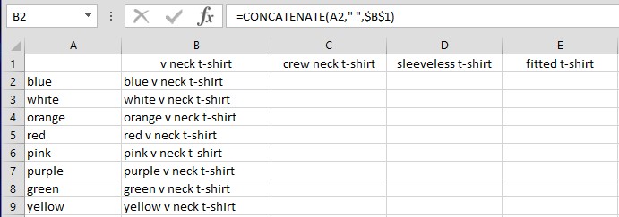
Just remember to ‘fix’ the cell containing the variable you DON’T want to change, in this case, B1 – ‘v neck tshirt’.

Also, be aware that =CONCATENATE will just join together whatever is in each cell, so if you need to add spaces between the strings (i.e. between “blue” and “v neck tshirt”), you can either:

• Add this into the cell you’re referencing, i.e. add a space before “v neck tshirt” in cell B1
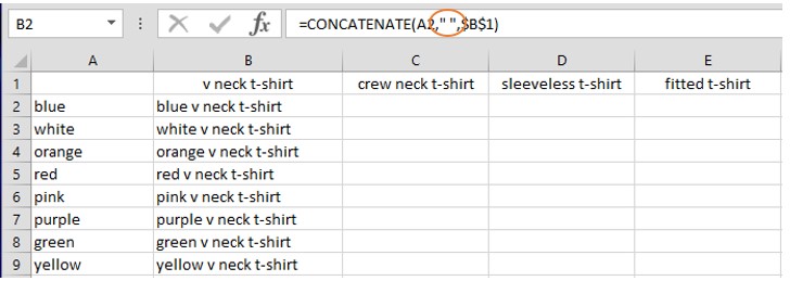
• Add the space into the formula as if it was a word you wanted to concatenate. I.e., add a space in between speech marks into the formula between A2 and B1 as below:

Saving more time – Applying the same formula to all cells

Once you have your first column of concatenated data, you can also drag the entire formula to the right to populate all the other cells in the sheet, but you’ll need to apply some more complex fixing of the cells to do this. In this instance, we’d need to:

• Work out which elements of the cells referenced in our first concatenation in B2 should be fixed in place, and which should be free to change.
• In this instance, the basic formula in B2 is =CONCATENATE(A2,” “,B1)
• If we want to drag this formula in B2 across into C2 and beyond, we’d need to change the B1 part of the formula to fix the reference to row 1 in place (to make sure we’re always referencing a t-shirt), but allow the reference to column B to move (so that the specific t-shirt type can change when the formula is dragged)
• To do this, we’d need to click next to B1 in the formula and keep hitting the F4 key until just the “1” part of B1 has the $ sign in front of it. It should look like this: =CONCATENATE(A2,” “,B$1)
• Similarly, we’d need to change the A2 part of the same formula so that the reference to “A” remains in place (to make sure we’re always referencing a colour), but allow the reference to row number 1 to move (so the specific colour can change when the formula is dragged)
• Again, to do this, we’d need to click next to A2 in the formula and hit the F4 key until just the “A” part of A2 has the $ sign in front of it.
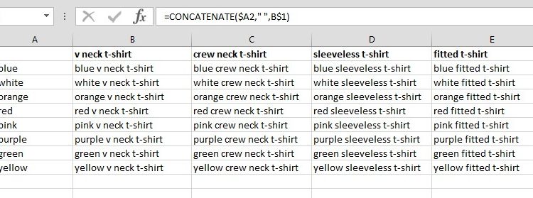
• The formula in cell B2 should now look like this: =CONCATENATE($A2,” “,B$1)
• This means the entire formula can be dragged down to fill in each colour variation for ‘v neck tshirt’, and also across to fill in each t-shirt variation for the colour blue.

This sounds pretty complicated, but is actually fairly simple once you get the hang of fixing different aspects of the cells referenced in a formula. It has the benefit of being able to write a single formula that then populates the entire workbook instantly:

Bonus! Getting all this data into a single column

So now you have these columns of different colours for each t-shirt type, you’ll probably want to run them through Google’s Keyword Planner and start getting search volumes for them, in which case you may want to keep them in separate columns for each t-shirt type. But what if you wanted to combine all the data into a single column?

Well, you could simply copy and paste each column into a new, single, combined column (using paste values to ensure you just paste what’s written in each cell rather than the formula itself). This is fine and doesn’t take too long if you only have a few columns of data, but if you’ve used the concatenate formula to create 10s or 100’s of columns of data, you may want a less time intensive solution.

We can do this by using the =INDEX formula to lookup each of the values within the complete array of cells you have, and transpose them into a new single column.

Here’s how:

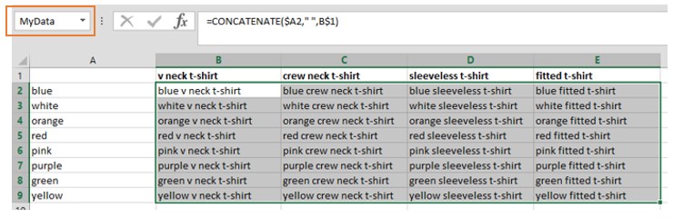
1. Firstly, you need to select all the data you want to combine into a single column and give it a name. You can do this by highlighting the data, going to the Name Box in the top left corner of the screen, inputting a name, and hitting enter. The name can be anything you like, in this instance I’ve named the data ‘MyData’:
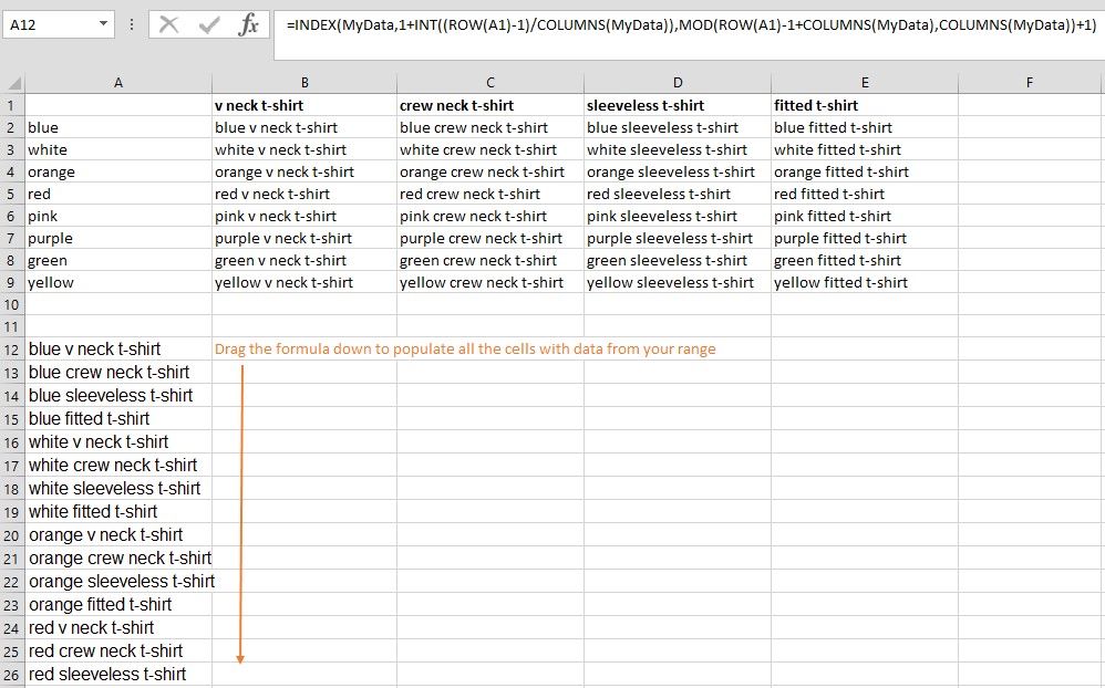
2. Next, just copy and paste this formula into the cell where you want your combined column of data to start. Again, if you’ve called your range of data something other than “MyData”, you’ll need to replace this in the formula with the name of your range:
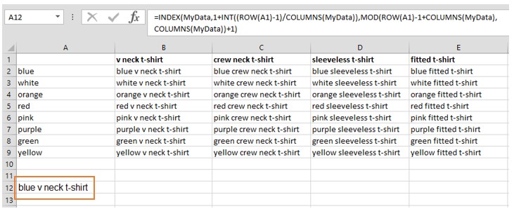
   =INDEX(MyData,1+INT((ROW(A1)-1)/COLUMNS(MyData)),MOD(ROW(A1)-1+COLUMNS(MyData),COLUMNS(MyData))+1)
3. Once you’ve pasted the formula in and hit enter, you should see the data in the first cell of your range appear, in this case, “blue v neck t-shirt”:
4. You can now just drag the formula down until all the data in columns you’ve created with =CONCATENATE is present in this new single column:
5. You can keep dragging this formula down until all the data from your range is present in this new column.

 

We hope you find this guide to using =CONCATENATE for common SEO tasks useful, it’s quite a basic function but can be a real time saver for a lot of monotonous tasks. We’ll be continuing this set of guides on Excel For SEOs in the coming weeks, so if you have a task that’s taking up loads of time and you think might benefit from some Excel wizardry, let us know!